Automotive Tire Pyrometer Project
By Daniel Hankewycz, Mouser Electronics
Licensed under CC BY-SA 4.0
Overview
The pyrometer measures the temperature of a tire. The copper probe is jabbed into the tire itself, between the treads. The idea is that the probe tip should be about 1/16"-1/8" embedded into the rubber for good heat conduction. As long as tires are not extremely worn, then there should be plenty of rubber (1/4"-3/8") before you would poke through and puncture the tire. Some basic theory on how the components work will lay the ground work for System Build Up.
Step 1: Thermistor Theory
Thermistors are devices that change their electrical characteristic in response to temperature. Like the name suggests, resistance is the main characteristic that is dependent to temperature with these devices. Thermistors are very common in temperature applications because they provide high accuracy at a low cost.
Most thermistors follow an exponential relationship between resistance and temperature. The graph above shows the difference between a negative and positive coefficient thermistor; often abbreviated NTC and PTC. The main difference between the two being that NTC shows an inverse R-T relationship and the PTC shows a direct relationship. For this project I chose an NTC thermistor for a wider temperature range and also because they tend to be a bit cheaper.
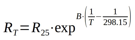
The equation above will produce the exact R-T curve for a Vishay NTC thermistor. Note the constants B and R25 within the equation; these values are specific for each thermistor. The R25 is the resistance of the thermistor at 25ºC. B has units of Kelvin (temperature), and relates to how quickly the graph drops off. Both of these values will be given to you in the component's datasheet. Keep in mind T is in units of Kelvin which is simple to convert from Celsius since Kelvin=Celsius+274.15. We will use these values and the RT equation in the next step to make some plots and tables to help us read the temperature with the microcontroller.
Step 2: Thermistor Reading Technique
So we have this component that reacts to temperature, but how do we actually read it using a microcontroller? The basic concept is called a voltage divider, and it uses the idea of series resistors having the same current.
The voltage divider is a very common circuit, found in almost all electronic designs. Any time two resistors are in series with one another, the voltage over one will always have a ratio of the total voltage over the pair. In our case we are using the fact that the thermistor resistance RT will be varying; therefore, the voltage drop over RS will change accordingly. This is similar to a potentiometer except a potentiometer allows full range to either VCC or GND because one of the two resistors can drop to nearly 0Ω. In our case, we can't “sweep” all the way to GND because of the constant RS value. The equation above shows how we can determine the voltage over RS as a function of RT.
The nice thing about this equation is that we can physically measure VRS using the ATtiny84's built in analog-to-digital converters (ADC). Once we have that, it's simple enough to solve for RT and use the equation from step 1 above, Thermistor Theory, to find our temperature. The only problem is that a microcontroller isn't good at doing complex math, so we have to use an alternative method of calculating the result.
Step 3: Function Interpolation (approximation)
The graph above is the resulting temperature vs. ADC curve when I combine the equations from steps 1 and 2. In order to calculate all values on the graph, the ATtiny84 would have to compute a natural log as well as floating point division. Since neither of those tasks are strong points for the 8-bit microcontroller, I looked to something that it is good at: memory look-up.
Reading from memory is fast, but in the case of the ATtiny84 it can still be resource expensive. The ADC on the chip returns a 10-bit value which can range from 0V to VCC. If I were to store the entire graph in a lookup table it would take 2048 bytes, which is 25% of the ATtiny's flash memory. Keep in mind that I am going to need some of that memory later on for character strings to generate menus. In order to make this task easier, engineers often use a technique called “function interpolation.”
The most common way of interpolating a function is to use line segment approximations of the original curve. In the image above (ADC to Temperature), the purple line is the theoretical temperature curve, and the green line shows the line segment approximation. I chose to quantize the graph by dividing the independent variable into 32 segments. Each segment can be represented as a straight line with a given slope and y-intercept. This helps combat the memory issue because now I just have to store two arrays with 32 elements each. The final implementation of the look-up table (LUT) will use 16-bit integers. This means that I will only use 128 bytes of flash in comparison to 2048 bytes if I were to store every value of the function.
Function interpolation drastically reduces memory resources, but as the image above shows, it does reduce accuracy in the non-linear regions. This imprecision can be avoided as long as we select a proper RS value that drives the linear portion of the curve within the selected temperature range (50-200ºF). There’s a spreadsheet document named ntc_thermistor_lut_generator.ods in the Resources section that contains all the calculations that I used to determine my values for the LUT. The spreadsheet allows you to use different thermistor characteristics as well as experiment with different RS values. It also generates the plot you see above, along with the percent error.
Step 4: Fixed Point Arithmetic
Representing integer numbers like 2, 5, and 17 in binary is simple. Conversely, what if you wanted to represent fractional values like 0.5 or 1.1?
To convert a binary number to decimal, we take the base value which is 2, and raise it to the current digit’s location from the radix point (radix being the general name for a decimal point). The same logic applies to digits to the right of the radix point, except now their exponent has to be negated. For instance, a 1 located two bits to the right of the binary point would have decimal value 2-2=1/22=1/4=0.25. The graphic above (8-bit binary 4.4 fixed point representation) shows this same calculation, but provides a more physical explanation than can be put into words. In the case of the pyrometer readout, we will have to make a decision as to how many bits of precision will provide sufficiently accurate data without excessive memory usage. The spreadsheet (<fn>=ntc_thermistor_lut_generator.ods) for the LUT in the Resources section contains a self-generated plot of the fixed point and interpolation error that is incurred throughout this process.
Step 5: Voltage Regulation
Since this device is battery powered, we need an efficient voltage regulator. The typical LM78xx series of linear voltage regulators simply wouldn't work since they require around 40% more voltage than their target output. I also didn't want to go with a switching power supply since that requires a high part count, and therefore higher cost. The next best regulating technique is to use a zener diode shunt regulator.
Zener diodes are device that are designed to operate quite efficiently in their break down region. A typical diode will start to build up heat once in the breakdown region, but a zener diode's characteristics allow it to hold the voltage at near constant. For this reason, a zener regulator is a perfect application for a power device. The only critical part to designing a good zener regulator, is to make sure that the diode is always operating in the breakdown region. This can be achieved by simply putting a resistor in series with the diode. The circuit in the figure above shows how the ideal voltage drop across the resistor will always be 1.5V. If I want at least 5mA of current to flow through the diode, then I just need to use ohms law to solve for the resistor value. Here, I used 10mA just to give myself a bit of wiggle room, and ohms law says R=1.5V/10mA=150Ω.
We would love to hear what you think about this project; please tell us in the comments section below.


